Sequential Domain Reduction

Background

Sequential domain reduction is a process where the bounds of the optimization problem are mutated (typically contracted) to reduce the time required to converge to an optimal value. The advantage of this method is typically seen when a cost function is particularly expensive to calculate, or if the optimization routine oscillates heavily.

Basics

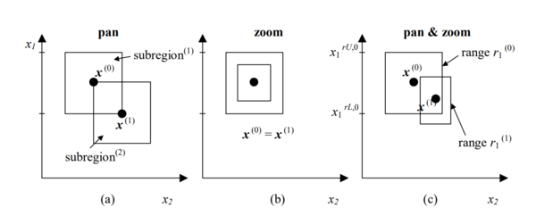
The basic steps are a pan and a zoom. These two steps are applied at one time, therefore updating the problem search space every iteration.

Pan: recentering the region of interest around the most optimal point found.

Zoom: contract the region of interest.

Parameters

There are three parameters for the built-in SequentialDomainReductionTransformer object:

\(\gamma_{osc}:\) shrinkage parameter for oscillation. Typically [0.5-0.7]. Default = 0.7

\(\gamma_{pan}:\) panning parameter. Typically 1.0. Default = 1.0

\(\eta:\) zoom parameter. Default = 0.9

More information can be found in this reference document:

---

Title: “On the robustness of a simple domain reduction scheme for simulation‐based optimization”

Date: 2002

Author: Stander, N. and Craig, K.

Let’s start by importing the packages we’ll be needing

import numpy as np
from bayes_opt import BayesianOptimization
from bayes_opt import SequentialDomainReductionTransformer
import matplotlib.pyplot as plt

Now let’s create an example cost function. This is the Ackley function, which is quite non-linear.

def ackley(**kwargs):
    x = np.fromiter(kwargs.values(), dtype=float)
    arg1 = -0.2 * np.sqrt(0.5 * (x[0] ** 2 + x[1] ** 2))
    arg2 = 0.5 * (np.cos(2. * np.pi * x[0]) + np.cos(2. * np.pi * x[1]))
    return -1.0 * (-20. * np.exp(arg1) - np.exp(arg2) + 20. + np.e)

We will use the standard bounds for this problem.

pbounds = {'x': (-5, 5), 'y': (-5, 5)}

This is where we define our bound_transformer , the Sequential Domain Reduction Transformer

bounds_transformer = SequentialDomainReductionTransformer(minimum_window=0.5)

Now we can set up two identical optimization problems, except one has the bound_transformer variable set.

mutating_optimizer = BayesianOptimization(
    f=ackley,
    pbounds=pbounds,
    verbose=0,
    random_state=1,
    bounds_transformer=bounds_transformer
)

mutating_optimizer.maximize(
    init_points=2,
    n_iter=50,
)

standard_optimizer = BayesianOptimization(
    f=ackley,
    pbounds=pbounds,
    verbose=0,
    random_state=1,
)

standard_optimizer.maximize(
    init_points=2,
    n_iter=50,
)

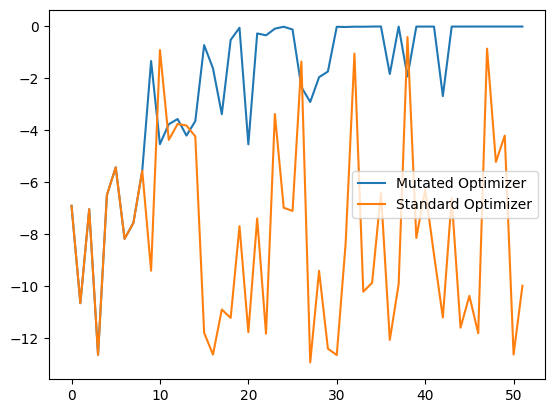
After both have completed we can plot to see how the objectives performed. It’s quite obvious to see that the Sequential Domain Reduction technique contracted onto the optimal point relatively quick.

plt.plot(mutating_optimizer.space.target, label='Mutated Optimizer')
plt.plot(standard_optimizer.space.target, label='Standard Optimizer')
plt.legend()

<matplotlib.legend.Legend at 0x23439267280>

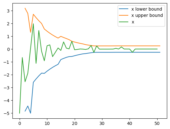
Now let’s plot the actual contraction of one of the variables (x)

# example x-bound shrinking - we need to shift the x-axis by the init_points as the bounds
# transformer only mutates when searching - not in the initial phase.
x_min_bound = [b[0][0] for b in bounds_transformer.bounds]
x_max_bound = [b[0][1] for b in bounds_transformer.bounds]
x = [x[0] for x in mutating_optimizer.space.params]
bounds_transformers_iteration = list(range(2, len(x)))

plt.plot(bounds_transformers_iteration, x_min_bound[1:], label='x lower bound')
plt.plot(bounds_transformers_iteration, x_max_bound[1:], label='x upper bound')
plt.plot(x[1:], label='x')
plt.legend()

<matplotlib.legend.Legend at 0x23439267fd0>